— an LSTM + CNN + Transformer Ensemble
TL;DR
Industrial IoT networks emit hundreds of multivariate sensor readings per second, and detecting cyber-attacks hidden in those streams in real time is a hard problem. In this project I trained three complementary deep models — LSTM, 1D-CNN, and a Transformer encoder — on the SWaT (Secure Water Treatment) dataset, and wired them into a Kafka-based streaming pipeline. Decisions are made by majority voting: an alarm is raised the moment at least 2 out of 3 models cross their thresholds.
All code and trained models on GitHub: github.com/mraknar/iot-anomaly-detection
The Problem
Three properties make attack detection in IIoT (Industrial IoT) particularly painful:
- Severe class imbalance. In SWaT, 96.21% of samples are normal and only 3.79% are attacks. Plain accuracy is misleading — a model that always predicts "normal" already scores 96%.
- Strong temporal dependency. The signature of an attack does not live in a single reading. It accumulates across roughly 10 consecutive sensor steps.
- Low-latency requirement. In a critical environment like a water treatment plant, the alarm needs to fire within a second or two. Offline batch analysis is not enough.
A single model struggles to satisfy all three at once. That is why I combined three different architectures with complementary strengths.
The Dataset — SWaT (Secure Water Treatment)
A public benchmark dataset collected from iTrust Lab's scaled-down water treatment testbed.

- 1,441,719 time steps
- 51 sensor / actuator variables (pressure, flow, level, valve states, etc.)
- Labels: Normal (0) and Attack (1)
- Class distribution: 96.21% / 3.79%
Preprocessing pipeline:
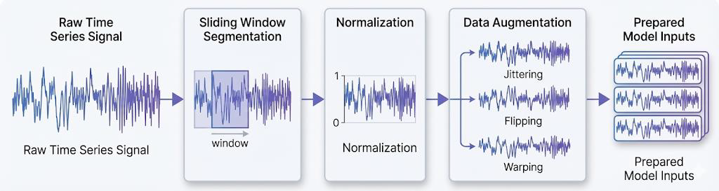
- Strip column names; drop timestamp and label columns from model inputs
- Min-Max normalization fitted only on the training split, then serialised to
scaler.pkland reused unchanged at inference time — this is the only reliable way to avoid train/serve skew - Sliding-window segmentation:
SEQ_LEN = 10, so each model input is a(10, 51)tensor - Stratified train/test split preserving the original 96/4 ratio
The Three Models
I deliberately chose architectures with complementary behaviour:

1) LSTM
Two stacked LSTM layers (64 → 32 units) with dropout. Its job is to capture gradual drift and long-term temporal dependencies in sensor behaviour. Behaviour: the slowest of the three to react at attack onset, but once it "wakes up" it does not miss attacks (high recall).
2) 1D-CNN
Two convolutional layers (64 → 32 filters, kernel size 3) + global max pooling + dropout. Its job is to catch local morphological patterns — short-lived spikes, sudden discontinuities. Behaviour: the most balanced precision–recall trade-off of the three.
3) Transformer Encoder
Multi-head self-attention (4 heads) + feed-forward block + global average pooling. Its job is to capture long-range, global interactions across the window. Behaviour: the fastest to react at attack onset — it can jump from probability 0.05 to 0.94 within one or two steps.
Training setup

- Loss: binary cross-entropy with class weights to penalise the minority class
- Optimizer: Adam (lr = 1e-3 for LSTM/CNN, 1e-4 for the Transformer) with gradient clipping
- 20 epochs, batch size 128
EarlyStopping(patience=7)+ModelCheckpoint(monitor='val_accuracy')
All three models reach ~99% validation accuracy offline, but the real story is in their different precision–recall profiles — and that is exactly what the ensemble feeds on.
The Pipeline — Real-Time Streaming with Kafka

Offline evaluation alone is an academic exercise. I wanted to see how the models behave in a real streaming scenario, so I wired up:
SWaT CSV  ──►  producer.py  ──►  Kafka topic  ──►  consumer.py  ──►  3 models + voting  ──►  ALARM/SAFE
                                  (Kafka + Zookeeper in Docker)
- Producer (
producer.py) — reads SWaT rows, serialises each to JSON, and publishes them to theswat_sensor_datatopic. The demo scenario sends 50 normal rows followed by 50 attack rows so the live transition from normal to attack is observable. - Kafka broker — Zookeeper + Kafka brought up via Docker Compose; the topic is auto-created.
- Consumer (
consumer.py) — listens to the topic, maintains a 10-step sliding buffer, normalises the data using the savedscaler.pkl, and feeds it as a(1, 10, 51)tensor to all three models in parallel.
The Decision Rule — Majority Voting

Instead of trusting a single model output, I empirically tuned three different thresholds:
| Model | Threshold | Rationale |
|---|---|---|
| LSTM | 0.30 | Noisy outputs but high recall → low threshold |
| CNN | 0.40 | Balanced — neutral threshold |
| Transformer | 0.50 | Very confident outputs → standard threshold |
Decision rule: alarm = (votes ≥ 2) — strict majority across three independent decisions.
This significantly reduces false positives compared to any single model, while the Transformer's early sensitivity ensures recall is not sacrificed.
Live Behaviour Observed
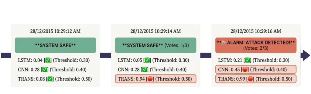
Normal regime (before the attack):
  LSTM  ≈ 0.03–0.10
  CNN   ≈ 0.25–0.35
  TRANS ≈ 0.05–0.10
  → 0/3 votes → SAFE

Attack onset:
  TRANS jumps first    (~0.94–0.99)   → 1/3 votes
  CNN  crosses shortly after          → 2/3 votes → ALARM
  LSTM joins last (cumulative drift accumulates)
This ordering is a perfect match for what the literature predicts: Transformers detect global deviation early, CNNs catch local morphology, and LSTMs add temporal stability. The ensemble combines three different time scales of evidence.
Resources
- GitHub Repository — all code, trained models, Docker setup, and the training notebook
- SWaT Dataset — available on Kaggle